MSc
This is the final product of the MSc I did at the university of East London (UEL) with Paul Coates and Christian Derix. It’s probably the least successful of the three big documents that I’ve posted (Undergrad 2 years before this piece and Diploma2 years after), but I learnt more than the outcome here lets on. Genetic optimisation is one of those topics that changes the way you view the world, but it does it very slowly. The ideas seep in and change every bit of your brain.
The intent was to “close the loop” and to make a GA that would use Ecotect for its evaluation, and GC for it’s geometry generation. Where David Rutten ended up succeeding, I failed.
I learnt a lot (set notation notation, C# programming, GA theory, how cad programme update cycles worked, a bit of graph theory) but learning it all at once meant that small things undid me. In the end the GA didn’t work (although in the write up I managed to convince myself that it did!). A few weeks after the submission date I took another look at the code and realised that I had a – where I needed a + and it worked perfectly.
This version of me is still way overconfident, my referencing is still terrible, but the work itself is much more complex. It spawned things like the genetic algorythms and pirates talk, probably had some hand in getting me a job at Autodesk, and set me up perfectly to supervise Go Kawakita’s Master’s thesis where he did what I was trying to do, but directly in Ecotect. Also, several of the illustrations from this piece ended up in Paul’s book.
The PDF (11mb) is here.
embedded and external optimisation with environmental evaluation
Ben Doherty
Submitted to the Department of Architecture in Partial Fulfillment of the Requirement for the Degree of Master of Science in Architecture: Computing and Design at the University of East London
September 2007
Abstract
This paper seeks to develop a genetic algorithm optimisation method that can be applied to parametric models by non-specialist users.
The dissemination of tools such as this is common in scientific circles with plugins for Matlab1 etc. but there has been no generic optimisation tool kit that has been made available to the architecture profession. As parametric modelling becomes more popular as a method of describing design intent and producing documentation, the ability to automatically modify designs within parameter limits, to find novel solutions or fine tune existing ones, becomes more attractive.
The solution was developed in Generative Components, and with a view to ultimately applying the principle of searching a design space for good quality solutions to the field of environmental design, there is potential to interface with ecotect.
Introduction
In order to provide a coherent workflow for analysis, there must be an easy flow of data from solution creation (generally geometry, but it could be fixed geometry and variable materials etc.) to analysis, and back again.

Fig 1. The export, import, interpret, action cycle
One of the main problems faced these days is that each software package has it’s own file format, and is essentially a closed entity that runs within a common framework (generally Microsoft Windows in architecture) and although Windows provides the means for packages to talk to each other whilst running (OLE2) it is very rare to see design packages implementing it for anything other than communicating with a database or spreadsheet.
This means that the workflow for analysis based design would generally be:
- To produce a potential solution that through a combination of perceived contextual pressures, aesthetic sensibilities and prior design experience[^3].
- To visualise the solution in a modelling package.
- To test its performance under certain conditions after moving it into an analysis package: This is a less straightforward problem than it might seem as issues that rarely surface in pure visualisation, for example, the unit attached to the arbitrary units (most cad packages use arbitrary units which have no real world equivalent until the user gives them one, so one package might export files assuming 1 unit to be 1 meter, and another might assume it is 1 millimetre), and numerous other minor but vital details.
- To interpret the results from the analysis package, which are then generally in the form of some sort of quantitative data, rather than a suggestion of the solution to a problem (that would require the package to recognise that there was a problem in the first place) and so require some interpretation by the designer.
- To start the process again with the knowledge that the designer has gained from the analysis of their initial solution.
This analysis loop is significantly faster now that it is being performed ‘in house’ by the designers themselves rather than being sent out to engineers who would take at least a week to complete an energy model, so now the cycle can be turned over two or three times a day at the beginning of the design process.
A method whereby the whole loop could be closed and executed without any of the complications of exports and imports could be very useful, and can be implemented in two ways.

Fig 2. Tools within a host application
The method that is prevalent in computer aided engineering (CAE) is that analysis and other non-geometry creation packages live within the main package as a plugin to extend the functionality of the host package. It is not uncommon for one plugin to be made compatible with several host packages3. The complexity of functions, cost per seat, and stability of the CAE market allows this to be practical.
Fig 3. Associative meta-data built onto base geometry
In contrast, architectural cad packages tend to be ‘stand alone’ and this interoperability is only just beginning to be addressed with standards like IFC4 (Industry Foundation Classes) and GBXML5 (Green Building Extensible Markup Language), these formats allow for the attachment of meta data and the capture of associativity, meaning that the six planes that comprise the cuboid that represents a wall, are not only associated with a line that defines the walls centre line, but also contain all the data that is relevant to the construction and performance of that wall. Unfortunately the standard way of moving geometrical model data around is still the DXF6 (Drawing eXchange File) file format which contains no associativity, and no meta data (it was invented in 1982, and has not been significantly modified since).
Of course, once one has one’s interface between geometry creation and analysis as seamless as possible, there is still the process of interpretation of the analysis data, and then acting upon it. This is where some sort of automated design process becomes useful. Without getting into the finer philosophical details of what design really is, if a design can be defined in terms of a system with some input parameters, and has some sort of measurable outcome, then finding the best solution is ultimately deterministic. For a very large search space, however, the time it takes to calculate the answer is longer than it takes to build a prototype of the solution and test it in the real world.
Fig 4. Applications that require export
If a design can be described in such terms, then it can be ‘optimised’. The word implies finding the optimum solution, however optimisation (making something be the best it can be) is a misnomer; in any non-trivial search space, finding the ‘optimum’ solution is spectacularly unlikely. It is important to remember that all of the optimisation techniques described below are really just improvement techniques that seek to move towards the optimum (i.e. make it better than it is now). Without an exhaustive search (complete enumeration) guaranteeing peak fitness is impossible (like requiring death to disprove immortality).
There are, generally speaking, two methods of solving a problem, computationally or analytically. These can be paraphrased as searching for the answer or going straight to it. Obviously it’s better to go straight to it but, if you don’t know where_ it_ is, that can be a bit tricky!
To solve a problem analytically there needs to be prior knowledge of the behaviour of the system being modelled. Generally an analytical approach is much faster once it has been defined, but it requires a formula to be defined which is often impossible if there are unknown behaviours involved
Briefly outlined below are some search methods for finding an optimum solution. The idea of search is easily visualised up to three dimensions (variables), but gets a lot harder to comprehend when one is trying to imagine what a 17 dimensional valley looks like!
“if it comes to a choice between spending another ten million years finding [the answer, or] on the other hand just taking the money and running, then I for one could do with the exercise”
Frankie – The Hitchhiker’s Guide To The Galaxy 7
complete enumeration
Fig 6. As the number of variables increases linearly, the number of solutions increases exponentially
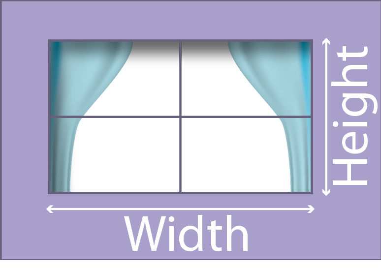
Fig 5. Example of window frame with two variable parameters
The most obvious and diligent method of examining a search space is complete enumeration. With the example of the daylight factor search given on page 24, complete enumeration would start at windowSize = 0 and increase in a given increment until windowSize = wallSize. Once this had been performed then the best solution could be taken from the history.
This sounds like a very reasonable way to do things, but when the complication of an extra variable is added in, say the height of the window, then we have squared the number of solutions to evaluate.
This very quickly gets out of hand and for 10 possible values for 1 variable we have 10 solutions, 2 variables, we have 100, 3 is 1000.
If each solution took a second to test then if we had a mere 8 variables it would take almost 3 years to evaluate all of them.
random search
By randomly picking values for parameters and testing them. If the performance returned is greater than the previous highest performing solution then that is stored. If its performance is poorer, the solution is disguarded. The process is then repeated for a predetermined number of steps, or until better solutions become very rare.
Searching randomly like this is not a very efficient way of finding solutions, it depends entirely on luck, but in a relatively complicated search space (more than say, 4 parameters) it is probably more effective than complete enumeration as the odds of the first parameter to be explored being the one that is most responsible for fitness are low.
hillclimbing
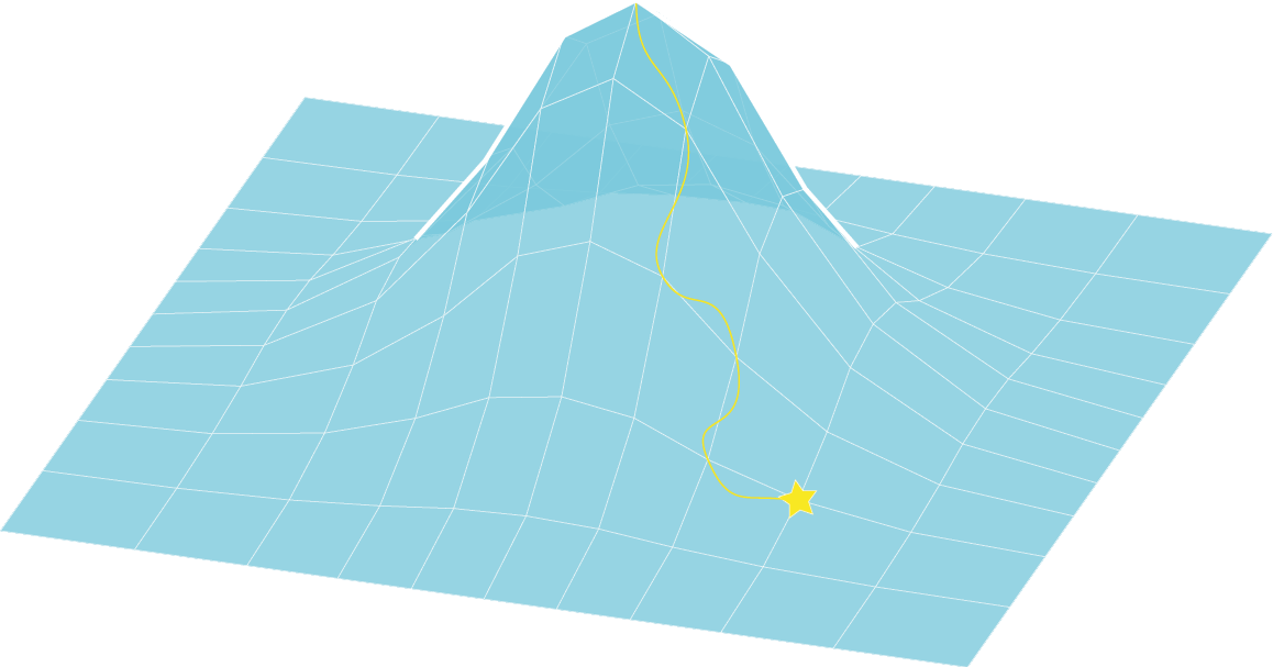
Fig 7. A fitness landscape with the two parameters plotted on the x and y axis, and the fitness plotted on the Z axis
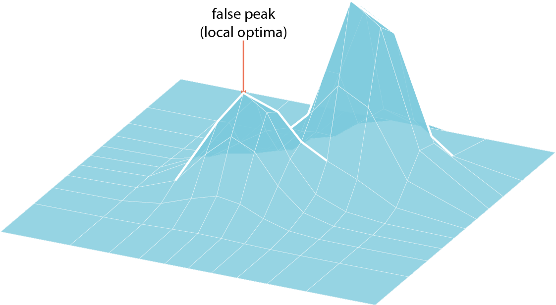
Fig 8. A fitness landscape exhibiting a false peak (a local optimum) and a valley
Hillclimbing starts off in the same way as a random search in that it picks a random point to start from, but once there, it tests the points surrounding it, and then moves to the neighbour with the highest fitness and again the process is repeated.
This can be visualised as being in very dense fog on a hill, so you test to see which direction is uphill, then move in that direction until every move you make would result in you going downhill.
Hillclimbing is susceptible to becoming stuck in local optima, if the algorithm finds a ‘peak’ it has no way of ensuring that it is the best solution, or merely better than the solutions surrounding it. For this reason, a simple hillclimbing algorithm is often put into a larger outer loop that makes it start again whenever this happens (called Random-restart hill climbing8).
genetic algorithms
The genetic algorithm (GA) is based loosely on the concepts of biological reproduction, and was first proposed by John Holland in 19759 as a method of optimization which would avoid the problems of local optima.
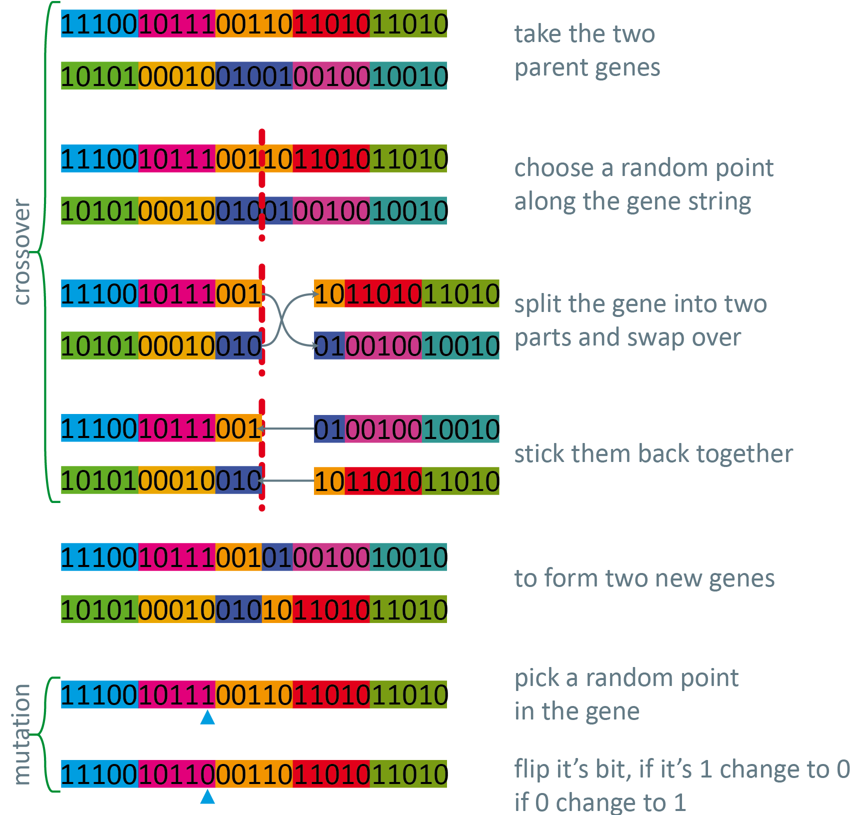
The basis of a GA is that there is a ‘population’ of solutions, which are then selected and ‘bred’ in a way that is weighted for fitness, the resultant population is then subject to a mutation (generally with a very low probability) and the process is repeated.
A simple GA is based on genes made up of binary strings, a simple list of 1 and 0. Initial populations are often generated at random, but they can be seeded with a percentage of genes that are know to be fit in order to give the system a helping hand in a large search space.
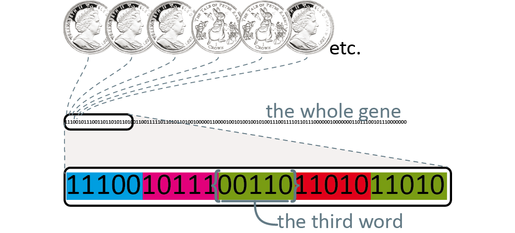
Fig 9. Defining a gene string
This is broken down into finite chunks of bits, which are then translated from base 2, back into base 10 to serve as parameters for a model.
The model is then tested with these parameters and a fitness is then assigned to that particular gene. It is important to note here that fitness is not defined in the athletic sense (running speed), or even the biological sense (number of viable offspring), but simply in terms of how well the system performs under those particular parameters.
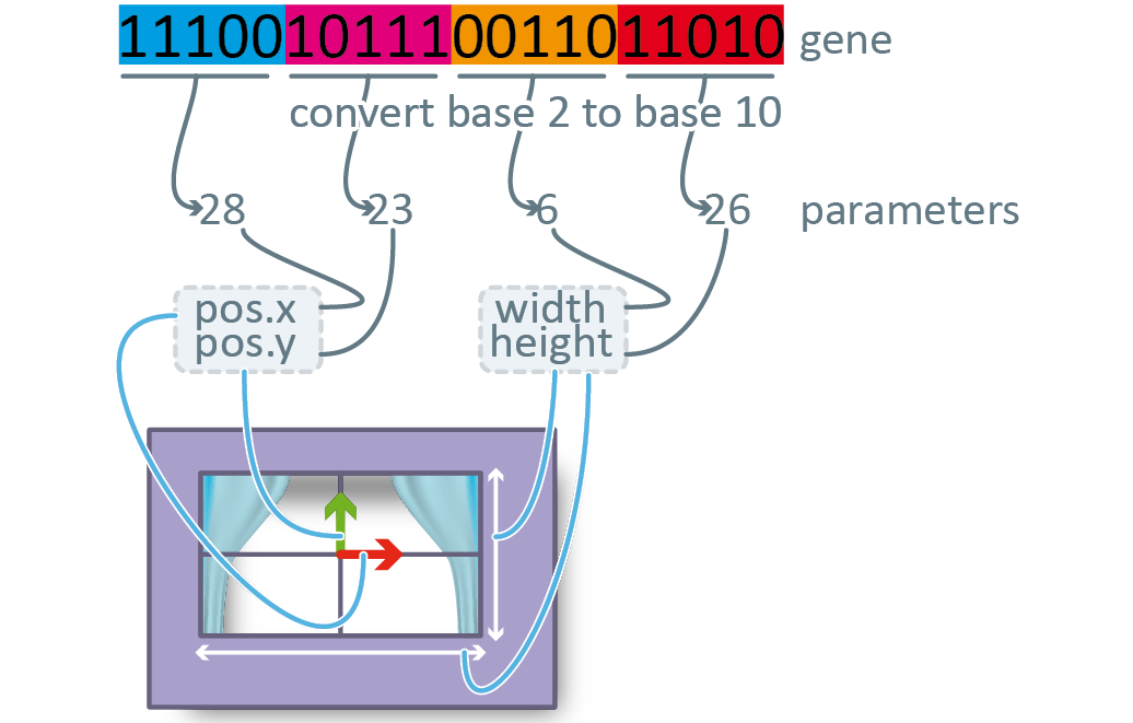
Fig 10. Translating a genestring back into integers to be applied to the parameters of a model
Now based on those assigned parameters the genes are ‘bred’ by crossing them over based on a probability weighted according to their fitness.
There is a large amount of borrowed biological terminology used in describing genetic algorithms. The Darwinian roots allow GAs to be understood fairly comprehensively by users with secondary school biology training, rather than having to have a significant mathematical grounding to even begin to comprehend the processes embodied.
Along with the design of the fitness function (which is covered below), the selection method is the most technical part of the process. The concept of selection is familiar to us all from wildlife documentaries, where the weak members of a herd of zebra are killed by the lions, and the stronger ones survive to have children.
There are many selection processes, but one of the simplest is roulette wheel selection10. The theory behind this is that it is possible that every gene, irrespective of it’s fitness in it’s current configuration, may well have some ‘genetic material’ that will make a worthwhile contribution to the genepool. So it would be foolish to simply pick the two highest performing genes from the pool to breed, as this would cause very rapid convergence on a local optima. If one imagines a GA roulette wheel, the slots on this roulette wheel are not numbered sequentially like on a traditional wheel, but are assigned according to the relative fitnesses of the genepool, so if a particular gene is twice as fit as another, it will have twice as many ‘slots’. This means that when the roulette wheel is spun, it could well land on a very unfit solution, but it is far more likely for it to land on a fit one.
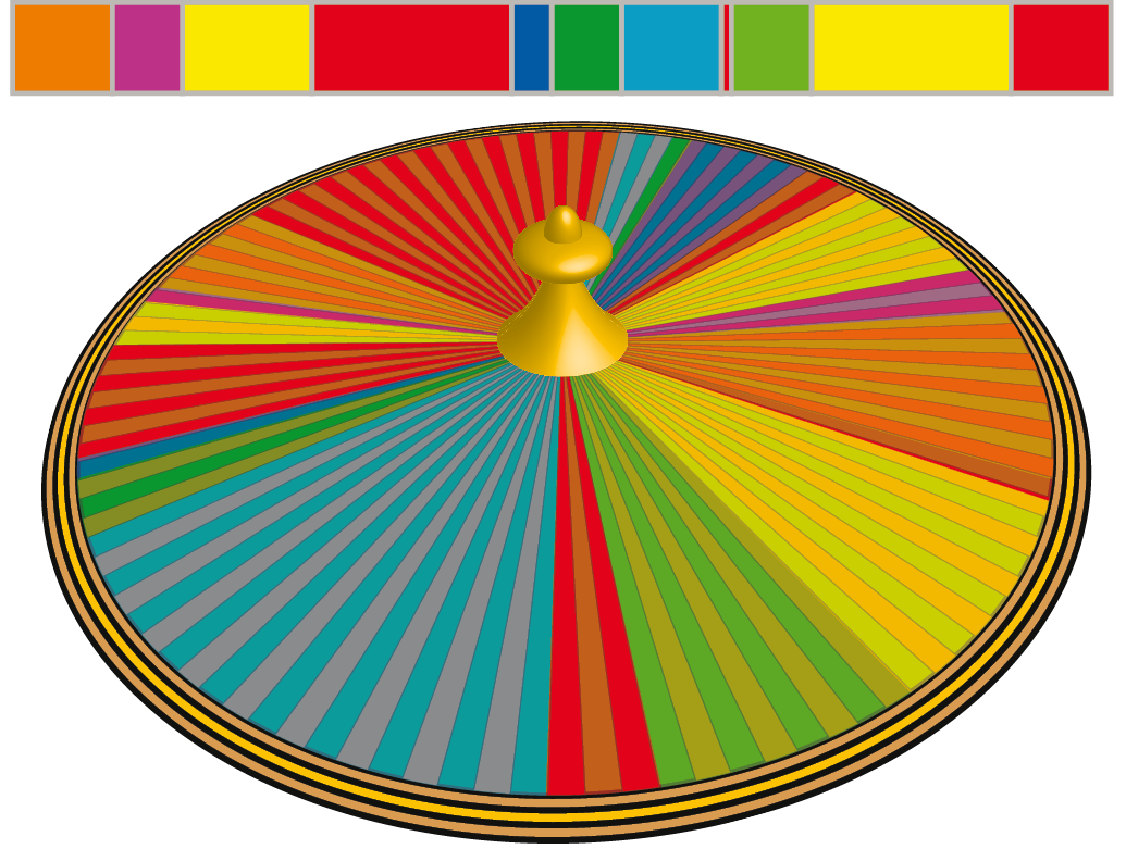
Fig 12. The roulette wheel. Note that the metaphor of the ‘slots‘ of the wheel mustn’t be taken too literally
I initially struggled with this concept and implemented a way that I thought was novel, but only works for problems that always produce whole number fitnesses (not a very common type of problem!) It was a too literal translation of the slots on the roulette wheel. It was a large array that contained the indices of the genes, repeated the number of times that the fitness dictated, so if the fitness of a small genepool were;
gene↓ ↓fitness
    0=2
    1=4
    3=1
    4=2
then the array would read
{0,0,1,1,1,1,3,4,4}
This worked well for integer fitnesses, and would probably be quite performance efficient for very large populations of such problems due to the ‘wheel’ array only being built once, and the selection simply being a random index into that array.
However, the traditional Goldberg roulette wheel works in quite a different way. The wheel is actually entirely metaphorical, and has no real relevance to the implementation.
I will explain my interpretation of this method with a little help from the Bash Street Kids11.
Given a population of possible solutions, each with their own fitness (here indicated by height) the first thing to do is to sum the fitnesses. This gives us a range to operate within.

Next we pick a random number between zero and the sum of the fitnesses to use as the finish line (in this case, represented by the height of the table top off the ground). Now we simply add up the fitnesses one by one until one of them is the one that causes the running total (of heights) to exceed the finish line value (height of the table top) that gene is then the one selected (the one that gets the cake!).
This works because the larger a gene’s fitness, the more likely it is to be the one that exceeds the limit.
There are various other selection methods, generally as variations on this theme, but with modifications, for example, to retain the best half of the population and to breed to replace the lower half.
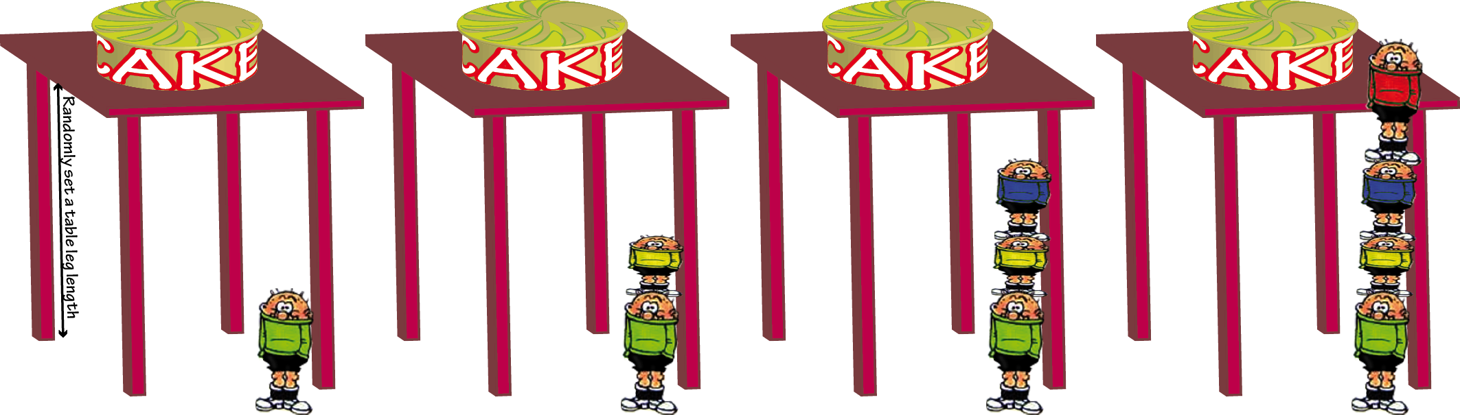
Fig 13. An alternative metaphor for roulette wheel selection – ‘first past the post’, or ‘who gets the cake‘ Pick a table leg length, and start stacking up your fitnesses, then stop when one of them passes the finish line!
The fitness function is where the ‘art’ is involved in designing a genetic algorithm, making a statement that produces a single value that will encourage selection for a particular trait that you are interested in.
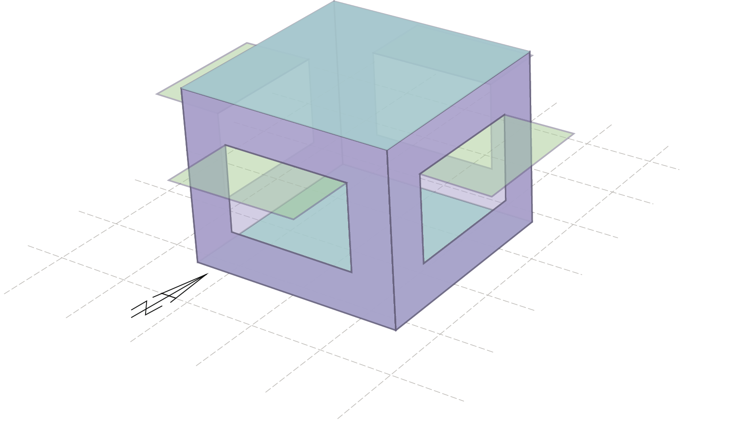
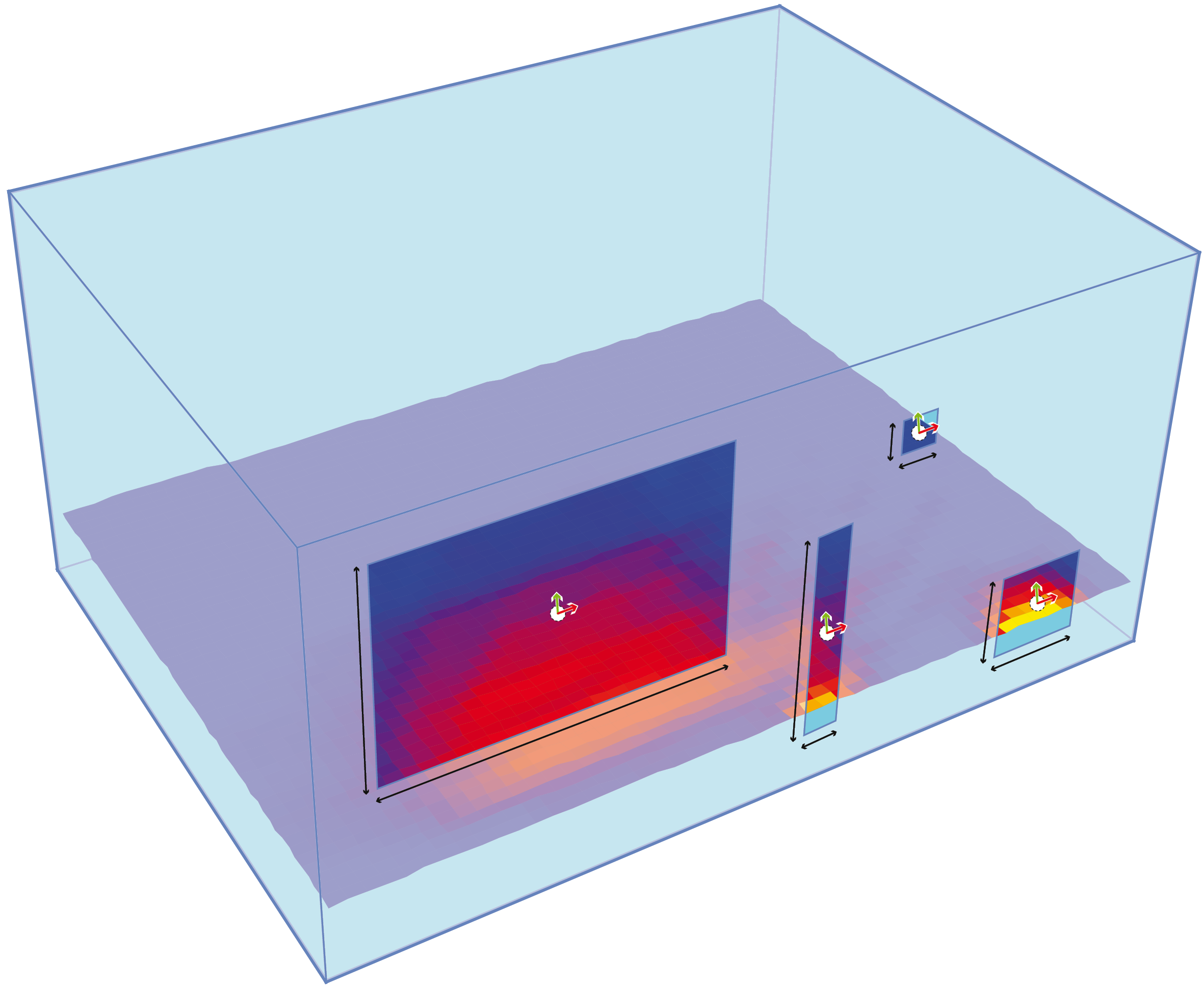
Fig 14. A test room showing possible window orientations
One interesting point to consider when testing the fitness is the role that the environment plays in a particular individual’s fitness. It is a little confusing to consider that there can be different environments, as surely the solution is just being simulated in the computer for use in a ‘real world’ environment, but really it is being simulated for use in a specific part of the real world environment.
The effect of environment on fitness is a profound as varying the particulars of a solution. For example, gills are a highly fit solution to breathing in an underwater environment, but in a city they prove totally unfit (hence there are no fish living wild in cities). This is why we see organisms (systems) developing into environmental niches.
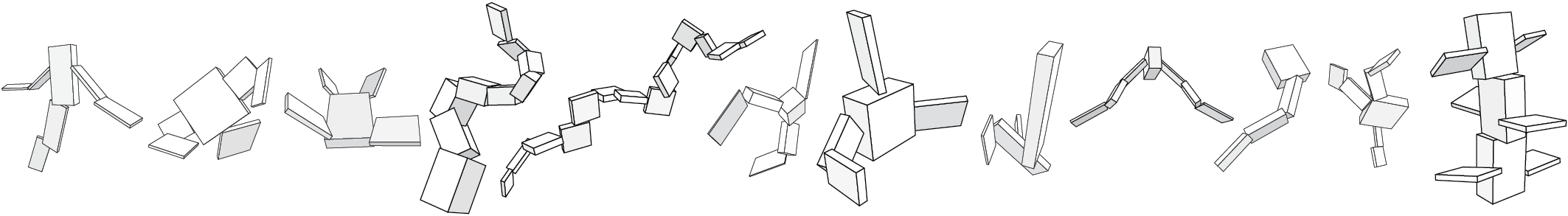
Fig 15. A selection of Karl Sims’ creatures that have been evolved for swimming.
Karl Sims’ Evolved Virtual Creature12 show this off elegantly as ‘creatures’ evolve for specific purposes depending on the parameters of the environment (friction, gravity, water viscosity etc.) even though they are all stemmed from the same initial body plan.
Figure 14 shows a possible test case: It is a room with four windows, one in each side. These windows are protected by an identical shading device. In each case, the parameters of the solution (the geometry of the shading device) are identical, but the environment differs (orientation), and as such they will exhibit very different fitnesses (ability to shade the window).

Fig 16. Additive colour mixing setup – by using three lights of varying intensities, any colour can be made
This can be formalised (using Holland’s descriptions) a little by taking the example of additive colour mixing.
It is probably wise to define some symbols to make reading the following a little simpler, as when Holland wrote ‘Adaptation in Natural and Artificial Systems’ educational in the United States was in the grips of the short lived ‘new math’ paradigm, with it’s overriding interest in set theory.
| α | the set of all possible solutions |
| A | one solution from that set |
| ε | the set of all possible environments |
| E | one environment from that set |
| ∊ | one member of a set i.e. g∊G |
| AμE | the fitness of a given solution with a given environment |
| τ | refers to the adaptive plan |
| Ω | is the set of operators that make up τ |
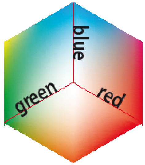
Fig 19. Three variables can be visualised geometrically as a cubic search space.
Given a set of solutions ‘α’ and a set of environments ‘ε’ they only meet at the test point and individual A is tested against environment E to give A_μE. This will then produce a set of corresponding fitnesses for the population specific to _E.
One of the key components in Holland’s definition of the GA is the ‘adaptive plan’ which he defines as the set of possible solutions(α) along with the genetic operators used to advance and modify those solutions towards a higher average fitness.
As the goal is unknown, the job of the search method is to attempt to make some sort of informed search for a solution based on the history of past tests and to infer the most productive step to take next. If τ is considered geometrically then the sequence of samples taken through that n-dimensional ‘space’ defines a trajectory through the search space (see the yellow line that traces a trajectory across figure 7). In GAs it’s not so significant, in other adaptive solutions it is essential (hillclimbing etc.) but in GAs it is just used to graph the history of the system to aid understanding of the system’s behaviour.
Returning to the colour mixing example, the parameters are the intensities of the three lights, between 0 and 100%, so if we only take integer percentages, then α is the 1000000 possible combinations of the intensities. If we ignore the complications of the colour of whatever we are projecting onto, then ε is a set of colours that we want to match.
So if we pick an E then the adaptive plan (τ) is α and the strategy (Ω) that you use to try and make A match E.
This is probably an overly specific way of describing things and leads to a significant amount of confusion, but is only really necessary when describing the workings of a GA in very precise detail.
If we were to control the intensities manually, then we would probably take an approach that was a hybrid of hill climbing and random search, possibly with an analytical element creeping in once we got a ‘feel’ for the systems behaviour.
Unfortunately there is no way that a computer can gain an insight into the workings of a system, (it can make generalisations about patterns, but it’s not the same as actually understanding).
A complete enumeration approach would be to fix the red and blue dials, and to then turn the green dial one click at a time to see if it made the colour match, then once all the possibilities of R=0, B=0, G=0-100 then all the possibilities of R=1, B=0, G=0-100 would be tried, and so on.
A random search approach would be to wildly turn the dials, and then write down the combinations that are better than the previous combinations. It is important to remember that there is no feedback between the fitness of the solutions and the next input sequence.
…and so on…
Case Studies
Fig 18. Site and location, note the shadow positions
Fig 17. An interior view of the building
The ‘Light House’ by Gianni Botsford is one of the most significant examples of computational architectural design with environmental driving factors. It is on an entirely enclosed courtyard site in Notting Hill, and as such, the only surface available for windows is the roof. Through detailed analysis, and many iterations, the plan and the roof paneling layout have been developed to work together to provide natural light right down into the lowest floor of the building. The courtyard was subdivided into voxels (3d cubic pixels) which could exist in a number of different states, for example, a number of different types of roof panel (glass, solid, fritted glass), void, or solid (floor or wall etc.). Solar data was provided using a combination of Radiance (a radiosity rendering package) and software developed at the Lawrence Berkeley National Labs. This data was then applied to the site and different; configurations of the voxel’s state13. The resultant (huge) search space was then explored using a genetic algorithm to produce a range of fit solutions. These solutions were then plotted to produce a ‘Pareto front’ to provide a heavily edited search space for the designers to choose from14. It would have been possible, given a very long time and an incredibly complex fitness function (containing factors that related to programatic issues etc.) to have developed the whole 3D configuration of the building using this method, but as project time was not quite infinite, the approach was mainly used on the roof. Quite significantly, the building was a real project that got built, in contrast to the majority of current projects that employ computational techniques which are terminated after competition stage, or are purely research endeavours.

Simple ecotect search script example

Fig 20. Sizing a window’s width to meet a specific daylight factor
This is an example of a very simple computational solution (a linear solver) to the problem of sizing a window for a room to provide a given daylight factor at a specific point. Using only a single variable, the program tests a small window size to see if it provides a sufficient daylight factor, upon finding that it doesn’t, it increases the size of the window and tries again, it repeats this process until it does pass the daylight factor test. There is only one parameter here, and it’s scope is very limited, so this approach works well. It could be solved even faster with a bifurcation solver, where it nibbles away at both ends of the parameters range and homes in on the solution rather than trudging towards it. This sort of highly constrained problem is ideal to be solved using solvers such as these, but when the search spaces become more complex then stochastic search methods become much more effective.
Parallels in other industries
Fig 21. Generic simplified baseline design
Fig 22. Effect of shape variables on nominal design (right)
In engineering computational design methods are far more widespread. This is probably due to engineers having a far higher general technical literacy, and there being far fewer ‘ephemeral parameters’ in most engineering problems. Most engineering design (and product design) packages work as a core onto which the user bolts the tools required to perform the tasks relevant to their sector, for example, sheet metal fabrication tools and finite element analysis tools for a designer involved in creating pressurised tanks, or complex surfacing tools and machine tool simulation tools for a designer working with the creation of plastic mouldings. Environmental design isn’t really a significant concern in the non-built environment sectors, but the principles of integrated analysis and optimization still hold to produce an ‘informed’ approach to the design problem, giving designers feedback on the validity of their decisions before they have to make real prototypes. (It is important to draw a distinction between environmental design, as in designing the environmental conditions of a space, and environmentally friendly design i.e. designing in general with conservation of natural resources etc. in mind) The Ford Research & Engineering Centre have used Altair Hyperstudy15 (a commercial optimisation tool) to improve the design of a turbo charger inlet manifold. The key criteria to search for was the flow velocity at the outlet. A number of variable parameters were identified in a notional model of the solution.

Fig 23. Section through the final optimised geometry Vs Baseline geometry
These were then tested at a variety of locations in the search space using computational fluid dynamics (cfd). The most promising solutions were then picked out for further testing. The actual process used for optimisation is not stated in the paper, but the solution seems to converge in five iterations. The final solution is not a radical departure from the nominal solution, but the form seems to have moved in an intuitive direction, and there is analysis data to quantify the design move16.
economics example

Fig 24. Goal Seek in OpenOffice Calc
The use of simulation and optimisation is widespread in economics. It’s implementation varies from very complex models such as agent based stock market simulations that include factors such as trader greed17, to very simple one dimensional problems in spreadsheets. It is possible to provide a spreadsheet with a formula and a variable and fixed value, then tell it to use it’s ‘goal seek’ feature to find the correct value for the variable. It is a complete enumeration method, and it stops at the first solution found, so for a complex equation there may be may solutions, but it will only provide one.
Packaged Tools
 For example the use of specialist animation software such as 3D Studio Max was the preserve of an elite few not too long ago, but nowadays it is fairly standard to learn it to a relatively advanced level on undergraduate courses. Over the last few years, more architects have been experimenting with creating their own tools, either as standalone programs, or as adjuncts to other packages. The possibilities for streamlining tedious processes, or performing generative processes make a set of custom tools very desirable. The popularity of programs like Generative Components, and the proliferation of publications such as AD – ‘Programming Culturesxi‘ can be seen as a barometer of this trend, and with the emergence of a bigger group of practitioners who are capable of making tools for themselves, an opportunity arises for people to make tools for tool makers. This allows the use (rather than the creation) of tools to propagate back down the skill gradient to allow non-specialist users access to the processes embodied in the tools, and also decrease the distance between the programmers and the users. Similarly to extreme programming, the fact that users have tools built by someone that they can email feedback to (if not shout ideas across an office!) changes peoples perceptions of the way they use tools. So instead of soldiering on with an inappropriate tool, users will simply request a new tool to do a job. This may ultimately end up far more integrated into the architectural workflow than we currently anticipate.
Unilever example
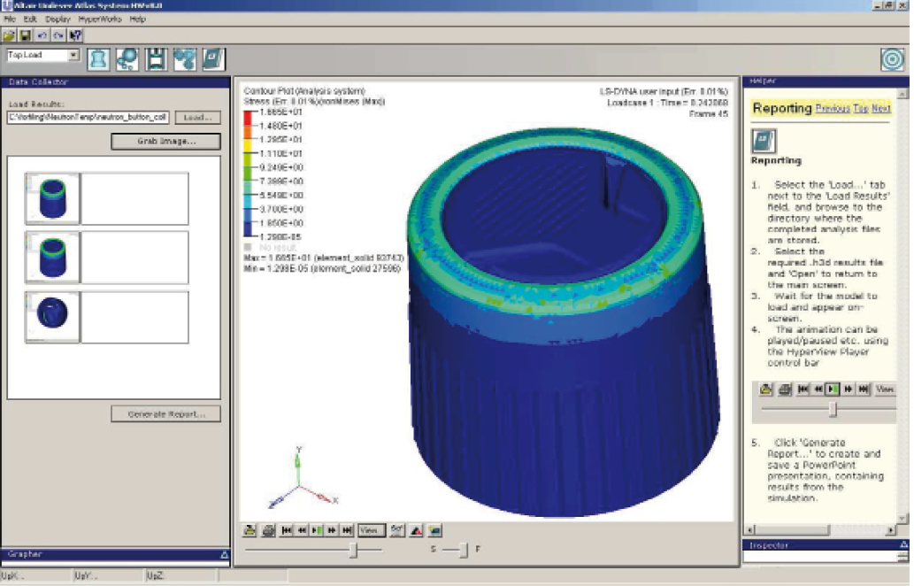
Fig 25. The Unilever custom interface for preparing analysis jobs and creating reports.
In designing the plastic moulding for the cap of the Lynx spray deodorant can18, the engineers at Unilever made extensive use of some fairly advanced optimization tools (Altair Hyperworks19) to decide on the structural arrangement of the cap. Once the methodology of the process had been established by the engineers, it was then packaged up within a standalone graphical user interface (GUI) ready to be used by the product designers. They were able to use it to prepare jobs to be sent off to a central processing server to test the feasibility of their proposals. There were two interesting components of this process. The design of the actual interface allowed a non specialist user base to access advanced CAE tools without a significant amount of training, and with out it being necessary to understand the underlying process.
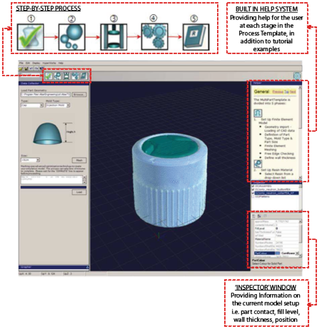
Fig 26. Supporting a streamlined workflow, accessible to non- specialised users
The interface hides all the unnecessary tools, and condenses the steps required to set up the analysis and produce reports into easy to use buttons. Also, the the stand alone interface doesn’t actually contain the analysis package; a complex analysis package, that can have a significant per licence cost implication, therefore makes it potentially prohibitively expensive to licence a large user base. Instead the interface contains only a system that prepares an encapsulated data package to be sent to be queued on the server which runs the analysis. As far as the user is concerned, the analysis can be treated as a black box that, given certain inputs, will behave in a certain way, but requires no understanding of the processes being performed. This is very similar to the workings of a modern car, where, in order to operate it, the driver has only to understand the interface (steering wheel, pedals, etc.) in order to produce an output (movement), and requires no knowledge of fuel flow fluid dynamics, or engine block metallurgy.
method of implementation
In order to create a design optimisation system for architecture, it must live within a package. For the reasons described above, creating another import export cycle is out of the question.
There are a number of factors affecting the choice of base package to extend. The primary concern is that there should be a parametric interface already implemented in the system, since one of the driving theories behind this project is that it should be extensible by non-specialised users, so that rules out Autocad (the most commonly used application in architecture) and most other CAD packages. It also rules out doing the whole project within ecotect as the geometry creation tools are fairly rudimentary.
Archicad already has a link with ecotect, and it has a rudimentary parametric modelling setup, however solutions must be programmed rather than modelled, using the embedded scripting language (gdl), and the possibilities for freeform geometry are somewhat limited. It would also be possible to implement it in an animation package such as Maya, 3D studio Max or Blender, as each of these has it’s own scripting language (mel, maxScript, and Python respectively) but there is a perceived lack of precision, no built in parametric interface, and no ability to ultimately produce drawings.
The only two real contenders therefore, are Digital Project and Generative Components.
Generative Components (GC) is Bentley Systems parametric and associative modelling package, it extends the base package of Microstation by adding a layer of tools for capturing design intent rather than simply ‘dumb geometry’. It is quite a young package (only officially launched in August 2007), but it had a large number of geometry tools. Most importantly, it has a very open and scalable programming interface that allows access in numerous way20.
Digital Project (DP) is a modification of catia; it uses the catia core to provide the geometry engine and then augments it with additional tools specific to architectural needs. Dassault Systemes (catia’s parent company) refer to an industry specific suite of tools as a ‘workbench’ so DP is the architecture workbench, but it is missing many of the tools that make catia so famous as they are included in the mechanical workbenches. It is overall a much more polished product, but has a less open programming interface21.
The package chosen to extend was ultimately Generative Components, it’s open access to be able to program simple things meant that tasks such as assigning control parameters to a model was very simple, and it’s almost viral popularity in it’s pre-launch phase, implies good things for the future ubiquity of the package.
programming approach
As already stated Generative Components allows several levels of programming interface. At it’s most simple, it allows properties to be entered as expressions, in a similar way to a spread sheet.

Fig 27. Generative Components supports spreadsheet style expression entry
It also has an internal scripting language called GCscript that is essentially based on C#, but has additional tools and built in methods that are specific to GC. Furthermore, it allows for code to be written without worrying about namespaces and headers, and to be edited and used within the program without being compiled.
transaction script "make a point" {
  double x, y, z;
  x = 1.0;
  y = 2.0;
  z = 3.0;
  Point myPoint = new Point(“myPoint”);
  myPoint.ByCartesianCoordinates(baseCS, x, y, z )
}
Fig 28. A simple GCscript block that draws a point in 3D space
At the most complex level, it is possible to write new features and GCscript methods externally in C#. These are much more difficult to write and test, but allow the programmer to call the full .net22 library to accomplish tasks.

Fig 29. Writing features and method libraries in C# is powerful, but much less flexible and accessible
Although there is all this programming possibility within generative components, I felt that it would be beneficial initially to write a genetic algorithm as a standalone Console application, both for exploration of the possibilities of the language, and to provide a benchmarking application to use as a comparison with the finished GC implementation of the GA.
The console GA went through several generations of it’s own before it was considered complete to a level that the logic embodied in it could be transferred to the GC environment.

Fig 30. Output from an early version of the console application.
The first iteration of the GA as a console application was written as a monolithic code block, mainly due to inexperience with the language, but as a proof of concept, and a way of tackling the problems involved in implementing the different parts of a GA in the .net framework. Features such as the ability to convert string representations of binary numbers into decimal numbers in one step, and being able to use the StringBuilder23 class rather than the String, which allows to access the gene’s string representation in a writeable way, made the process of actually writing the code significantly easier, but certain idiosyncrasies of the language took a while to get comfortable with.
This code was then reformatted into a single class, with methods. The Visual C# Express IDE has a very useful tool that automatically refactors a section of code into a method, there is still a little tidying up to do to make all the variables local etc. but this significantly clarified the process of writing methods in C#. However, the code still essentially followed a ‘functional programming’ approach to the problem.

Fig 31. Inheritance in this case is not applicable, but the HAS_A relationship is used
This approach wasn’t taking advantage of the power of object oriented programming, there was no inheritance, or encapsulation. I struggled for a while with the concepts of inheritance as applied to this problem, it eventually emerged that inheritance wasn’t applicable, as a gene is not a genepool with some additional properties (so the inheritance ‘IS_A’ relationship is not applicable), rather a genepool ‘HAS_A’ gene, so the constructor of the genepool instantiates an array of genes.
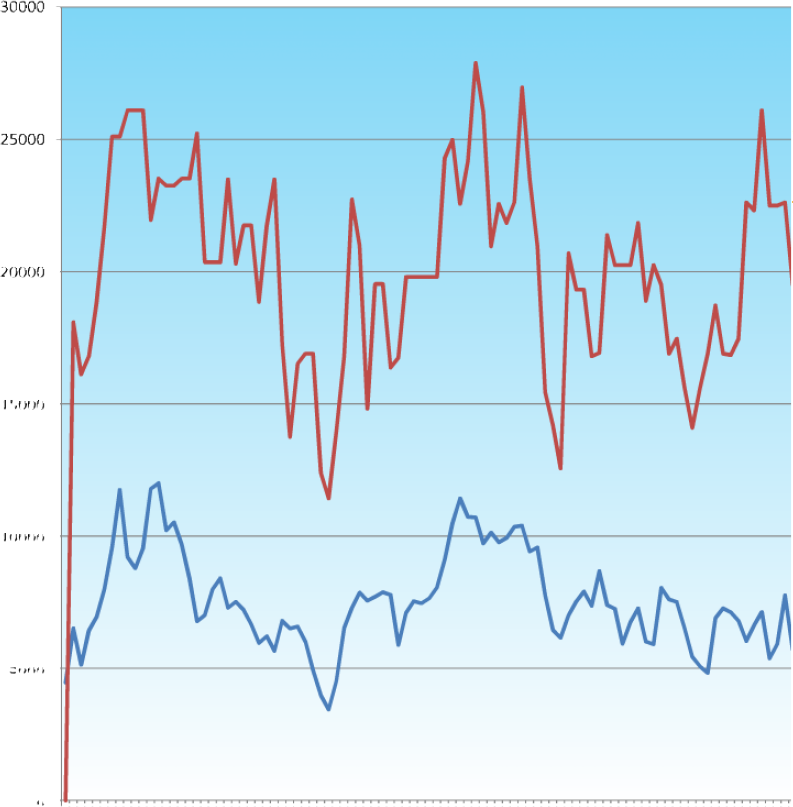
One of the challenges of creating a console based application is the graphical representation of the results. As the console is entirely text based there is no way of showing graphs without implementing a windows form or OpenGL based visualisation, the simple solution was to save to a text file24. This allowed the code to write the values of the best fitness and the average fitness for each generation out to the file, and then open the file in a spreadsheet and produce graphs immediately.
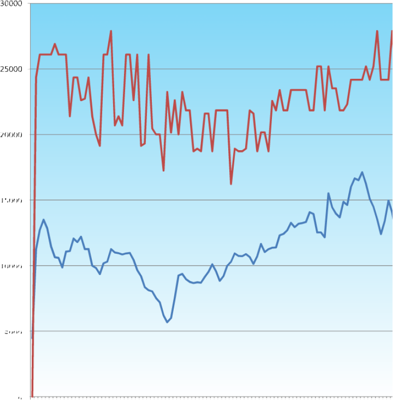
Having graphs of the performance of the GA proved invaluable in tuning the input parameters, and debugging the code. For instance, an early problem with poor convergence was traced back to a hard coded value for the mutation rate of 80% likelihood, but this would never have come to light based purely on text based output. The history graph has been used throughout the project as a way of assessing the systems performance. Given that it appears to be performing correctly, the console GA has also been useful as a yardstick to benchmark the performance of the GC GA.
These graphs are traces of the average and maximum fitnesses of the GA trying to achieve the maximum volume of a cube (simply L∙W∙H). They show the significant effect that the mutation rate has on the ability of the system to find a solution.
 |
|
 |
|
 |
|
 |
|
 |
|
 |
|
 |
|
The ultimate goal was to produce a fully packaged GC feature which users could access with almost no knowledge of the underlying process.

If we return briefly to the initial diagram of the import export cycle, the plan is to modify it to initially remove the analysis step, and then to remove the interpretation step from the loop and place it outside. This can be seen as the user delegating the task of designing, or searching for, a solution to the computer, and then making a decision on the result. So the process is now:

Fig 39. the design cycle augmented by an optimisation process
-

Fig 40. Initial understanding of the process required and scheduling involved in making GC GA Design a system with parameter ranges
- Design a method of quantifying it’s fitness
- Optimise that system using whatever process seems most appropriate (in Holland’s terms, pick your ‘adaptive plan’)
- Make a decision on whether to stop there and proceed with that solution, keep that solution in a selection of possibilities, or to discard the solution altogether and either run the process again, or redesign the process. It is interesting to note that the word design is coming up so much in this process when most people would consider the computational approach to be stepping away from design and into a more certain realm. This concept of delegation is again useful in that one becomes a meta-designer, or a manager of the process, and instead of designing the minutia oneself, one designs the system and process through which a design emerges.
The first model of operation that was proposed was: The user would provide a list of ranges to operate within, and a subdivision setting (to allow there be some idea of granularity).
The genetic algorithm written in C# would provide Generative Components with a set of parameters to evaluate by using them as inputs for a parametric model.
Generative Components would then do all the geometry related calculations, and pass a fitness value back to C#. If the GC↔ecotect link had been working, this is where GC would have sent the geometry that it had calculated to ecotect for analysis to evaluate the fitness.
Once a population of candidate solutions had been evaluated, the C# program would apply the genetic operators based on the fitnesses and provide a new population of candidate solutions.
Initially this seemed to be a very attainable goal, as the theory of creating some values within a set of ranges, and then testing them and passing back a fitness seemed very plausible, however, the reality is somewhat more complicated.Generative Components can execute scripts in two ways. To make sense of this a few definitions are useful.
- The base coordinate system (baseCS) is the point of origin and orientation on the otherwise infinite cad universe. It is also acts as the top node in the symbolic graph.
- Graph updates are called every time the user makes a change to the model, they are triggered as often as possible if the model is in dynamics mode, or when the user has finished editing if not. They can also be called from the code.
- Script transactions are a part of the ‘transaction list’, which is a linear sequence of events, which is generally used to record design history, but it is possible to write code (with loops and conditionals etc. as well as just a list of instructions) inside a transaction.
-

Fig 41. A more developed representation Graph functions are quite different to script transactions in that they are run every time a graph update is called. The model begins with the baseCS, and then recalculates the things that are directly dependant on that, and then progressively everything down the directed graph/tree until there are no more nodes left. Every time the update gets to a graph function, it provides it with updated inputs, runs the script, and then returns a new output.
Unfortunately the graph update problem means that the program needs to be run from the transaction list rather than being an ‘in process’ system that resides within a graph function. This loses the conceptual advantage of the transaction list being a method of capturing design intent in a historical manner. There is going to be an update sub-graph method available soon in GCscript, which will allow the graph to be updated selectively from one node down, but so far it is not exposed yet.
The problem is that in general, features are reactive rather than interactive. In that they take a set of inputs, and provide a particular output, so each update cycle, starting with the base coordinate system, every feature is refreshed, but if the GA controller is calling these graph updates from within itself then it will cause an infinite loop.
There are two things that are needed in order for a feature to work in a cyclical environment, a recursion guard, and an update subgraph method. The recursion guard is an outer conditional, which upon the feature being called is set to false, so that it is not entered in subsequent calls, then when the feature has finished performing it’s task, then it resets the switch to true.
The update subgraph method is required in order to start an update sequence with a starting object other than the base coordinate system. (update graph is really just an update subgraph, with a default start object of the base coordinate system.)
With these two things in place a feature’s influence can be stretched over several update cycles.
The only working example of this in practice is in a demonstration script that was written by Robert Aish & Jeff Brown which allows a rectangle to exert control over a group of points to ensure that they stay within its boundaries. If the points are being manipulated they can’t be moved outside the rectangle, and if the rectangle is being manipulated the points are pushed around to ensure that they stay within the boundary. This sounds trivial, but it requires a switching of the dependencies.
Although extensive progress was made in documenting the constraint solver in order to make it’s operation clear, ultimately the time constraints of this paper made it important to find another approach to solving the problem of implementing a genetic algorithm in Generative Components.
“Circular dependencies are far harder to explore than non-circular ones due to the feedback loops”
Axel Killian25
The most obvious way to begin making a GA seemed to be to take advantage of GC’s native programming language, and write the whole thing in GCscript. This has the advantage of it being possible to call a graph update without causing an infinite loop. However, there are several disadvantages to writing anything complex in GCscript. Firstly, there is no support for creating classes, or even types (VBA style26) which means that it is difficult to handle arrays of objects with several embedded properties, in this case, the gene, with it’s genestring, integer values, fitness, etc. so these all have to be handled in different arrays with corresponding indices. It is possible to make a C# based feature that has no geometry, and acts purely as a vessel for data, but as this technique (pure GCscript) wasn’t implemented, it wasn’t tested.
Also, for manipulating string based data, GCscript is hard work as the default C# string is a read only object, so it would require huge amounts of copying and temporary variables to perform a simple task such as switching a bit from 0 to 1.
| String implementation |
|
| StringBuilder implementation |
|
Fig 42. Initial understanding of the process required and scheduling involved in making GC GA
The solution that has been settled on for the time being is based in GCscript, but augmented by extending the native method library that is provided with GC (simple maths and geometry tools) with additional GA specific tools written in C#. It is an imperfect solution (for the reasons outlined above), but provides a usable intermediate stage until a fully packaged feature is made possible.
GCscript methods are proving to be very useful; they provide quick access to the .net libraries. This is useful for performing simple tasks such as string manipulation using StringBuilder rather than temporary variables, but also for extending GC for performing specific tasks.
As the C# based GCscript methods are added to the standard library with the existing methods, it is possible to test them by applying them to the console window, rather than building elaborate testing rigs. One simply enters the function as it would be used in a full program, complete with arguments, and it prints the result as it would be returned to the call in the program.

Fig 43. Testing a C# based GCscript method using the console
If a breakpoint has been set in C# this will invoke the debugger and allow the code to be stepped through as well.
One example of a solution that could only be provided by harnessing the .net library is creating a displacement map from a .jpg image. This is something that was undertaken more out of curiosity and a desire to test the extent to which the .net framework could be harnessed, than to solve specific need, but having created it, it could well become a useful tool for making topography surfaces, or managing free-form geometry.
It works by passing a file path to C#, which then loads the corresponding image, builds an array of the blue values (blue is an arbitrary choice, but if the image is grey scale, R=B=G27) and returns that array to GC to do with as required, in this case, to feed the Z values of a point grid. It would be possible to extend this to be a feature (possibly named BsplineSurfaceByImageMap, or something similar) that handled the geometry internally and returned the surface, but this is a great example of how useful C# based GCscript methods are in being able to prototype methodologies that could not be achieved within GCscript alone.
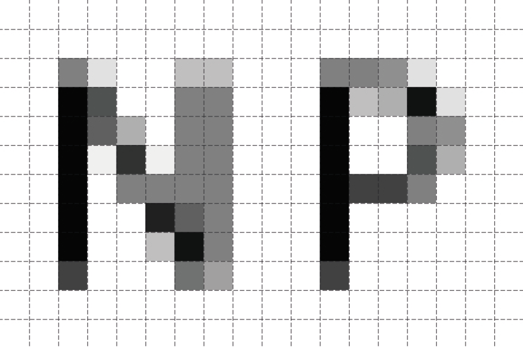
Fig 44. Grey scale bitmap input
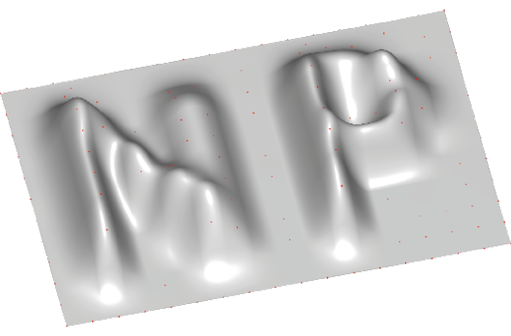
Fig 45. 3D surface output
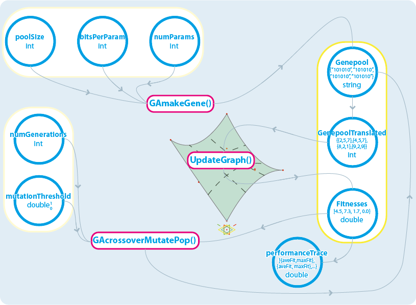
Fig 45. Scheduling and process diagram for GCscript solution with C# based GCscript methods
The updated model taking this new approach into account is as follows.
With the graph update as the pivotal point of the GA in terms of managing it’s operation, the procedures can be subdivided into three sets; those actions which need to be performed to initialise the system; actions that are within the optimization loop, that happen before the graph update call; and those after it.
These actions can be collapsed into C# based GCscript methods, in order to minimise amount of code exposed to the user, and also to try and improve performance since the externally written methods are compiled code, rather than dynamically interpreted. If we can’t make a black box, at least we can make a coherent and specific tool box.
Initially the gene pool size, and the details of the gene string are set, along with the number of generations to perform, are fed to the GAmakeGene() method, which instantiates an array of strings. This array is then read in and out of C# again to translate it into integers. This is the equivalent of the constructor in the console based GA, and could be collapsed into an even more dense method if specific data types were enabled.
Once there is a complete set of data to work from the loop is entered. The process of optimization can begin. There are two loops, an outer one that is run once per generation, and an inner one that is run once per population member. For each population member, the corresponding parameter values are read out of the genepool, and applied to the model, a graph update is called, and once the geometry is recalculated the fitness is read off (this fitness can be arbitrarily complex, from the volume of a cuboid, to the ratio of panel planarity, against solar gain).
This new array of fitnesses, and the array of genes is fed into the GAcrossoverMutatePop() method, which takes the genepool, the fitnesses and a mutation threshold. This now externally does all the selection, crossover and mutation associated with a GA and returns a new array of genes, ready for the process to start again.
Results
Until the GC ↔ ecotect linkage is implemented, the solutions to test are relatively trivial, as the real world evaluation is missing from the system. The solutions offer no real visual interest, so the results are presented generally as an overview of the problem, and the performance history graph.
benchmarking application
Due to the there being no need to communicate between packages, or complex geometrical and graphical calculations, the console based GA program has a hugely superior speed when compared to the GC implementation. This allows much larger populations and numbers of generations to be tested to ascertain the behaviour of the system, so that ballpark envelope values, at least for this simple system, can be found.
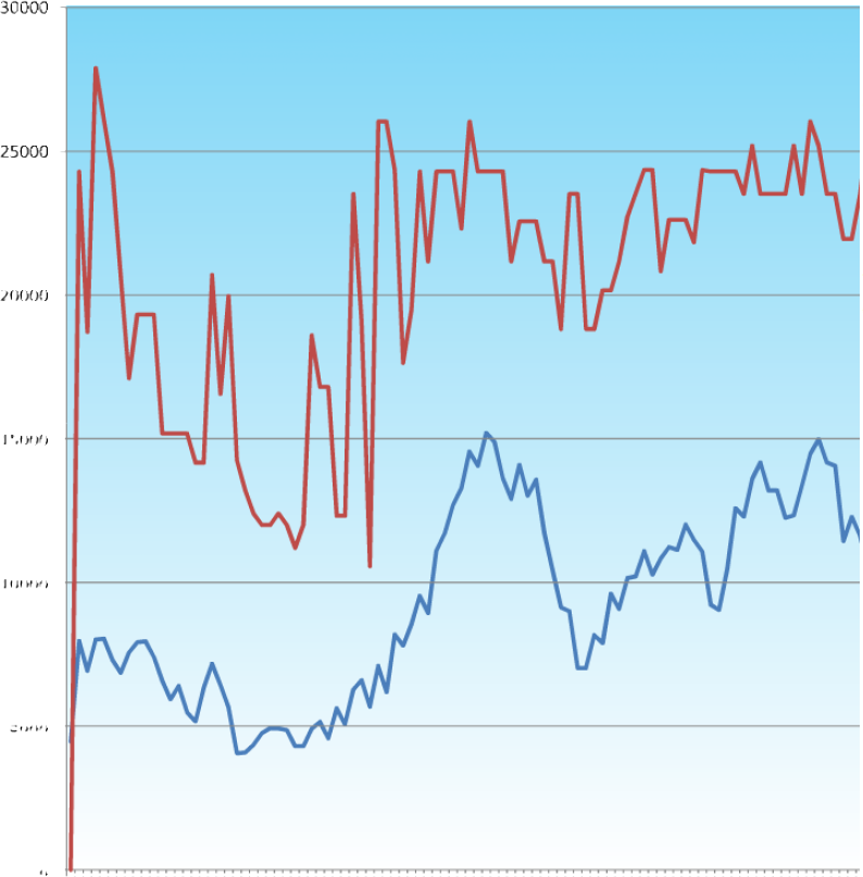
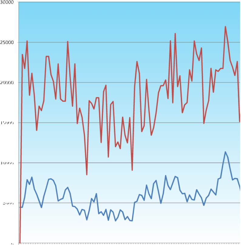
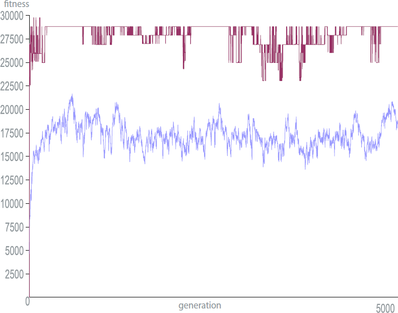
Figure 47 is the results of a very long run of the console based GA, again, the fitness function is the simulated volume of a cube i.e. L∙W∙H.
The other parameters are as follows;
- Population Size = 100
- Number of Generations = 5000
- Number of Parameters = 3
- Number of bits per Parameter = 5
- Mutation Rate = 3%
For a 5 bit binary number, the maximum attainable value would be 25-1 (minus 1 due to zero base) which gives 31 ∴ the largest volume and fitness would be 313 or 29791, which is found three times in the first 100 generations, but lost again, presumably due to an unfortunate crossover. With a mutation rate that the level that was suggested as sensible by the preliminary shorter runs shown earlier, nothing really disastrous happened, but also, nothing really great happened either.
One thing that I still don’t understand is the way that after an initial rise, the average seems to remain relatively constant throughout. Rather than rising to converge with the maximum fitness. It implies that there must be a constant supply of relatively unfit candidates in the pool too.

Fig 48. The trace of the fitnesses of the individual genes as the GC based GA optimises the volume of a cuboid.
This is the first instance of a GA running through GC with the augmented function library.
The graphs in GC follow the fitnesses of all the population members which allows us to see what the cause of a rise or drop in average fitness can be attributed to.
Again the solution doesn’t converge on the absolute maximum fitness available, but it does show a definite trend towards improvement.
The low mutation factor means that once the solution has converged (almost exclusively by selection and crossover) it is unlikely to jump out of it’s stasis to find a better (or worse) solution.
The parameters are weighted to reduce the very large bit length’s decimal equivalent to a more usable value, but the longer gene strings also provide a helpful amount of damping to provide protection against catastrophic mutation. In “1111“ there is a 1 in 4 chance that the mutated bit will have a significant effect, whereas in “1111111111111111“ there is only a 1 in 16 chance.

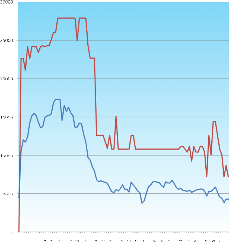
Fig 49. The trace of the fitnesses of the individual genes as the GC based GA optimises the volume of the intersection of two cuboids with a centroid with three degrees of freedom
This is the first of the more significant problems. There are twelve parameters; three each for the centroids in xyz space, and then three each for the cuboid’s dimensions.

Fig 50. Fitness graph of the solutions shown overleaf
The fitness function is defined as the volume of the intersection between the two cuboids, but if there is no intersection then the fitness is set to 0.1 (to avoid the complications that a zero fitness causes in the selection process).
Obviously the fittest solution will come from the two cuboids having the same centroid, and being as large as they can be. This produces a ‘ridge’ that the fitnesses can exist on if they are to produce the best results.
This search space is considerably larger, and as such the GA doesn’t find the perfect solution during the run, however, it does show significant improvement, and the population converges. The population is very small, so this total convergence isn’t so surprising, but what is interesting is the plateauing that is presumably caused by the crossover as sections of genetic material from fit solutions get selected several times and solutions switch in and out as a result. This seems a little odd as the crossover point is random.
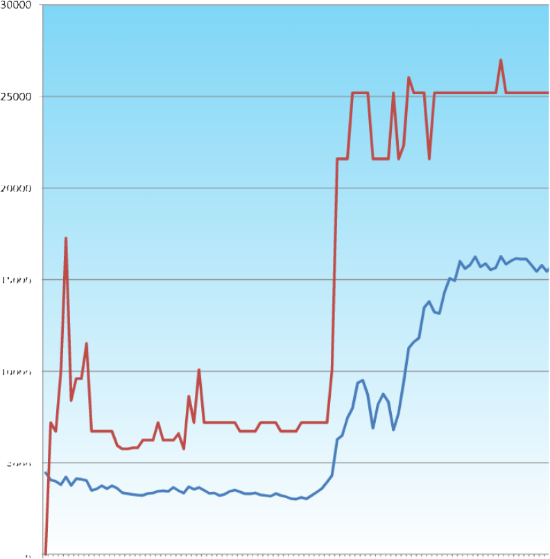
Overleaf is a visualisation of the 200 solutions produced by 20 generations of the GA running over the above problem. It’s interestign to note that the solutions seem to be keen on keeping the left cuboid static and moving the right one, this is an emergent strategy, and is not pre programmed into the system. Unfortunately the system finds an very good solution early on and then it is lost, presumably by crossover (parts of it, i.e. the large left cuboid can be seen in latter generations, but the rest of the gene encodes a zero fitness solution so it is removed from the population, losing that allele that could lead to a fit solution.) this is a good indicator that pure roulette wheel selection is perhaps a little too volatile for this type of problem, and a system that only replaces the least fit half of the population might be better.
Fig 51. 20 generation of a population of 10 members attempting to find the largest volume of their intersection. Generation 1 is on the left.
Discussion
Although the goal of a complete black box solution was not reached, the GCscript based solution provides a useful intermediary step in the implementation of optimisation in Generative Components, and given that the majority of GC users are architects or engineers, optimisation in architecture.
It is absolutely worthwhile pursuing further loop tightening strategies as genetic algorithms aren’t suited to all problems, so a solution toolkit which encompassed other search methods and some general solvers would prove very useful to the community.
Given the time taken to evaluate each population member when provided with a complex fitness evaluation (for example a dynamic cfd simulation), stochastic searches will always be less efficient than an analytical approach, however, if that analytical solution is unfathomably complicated then the ‘educated stab in the dark’ of a stochastic method will always win out over the ‘proper scientific solution’.
Without the ecotect linkage enabling the fitness function, a generic solution to the problems of analysing solutions with environmental driving parameters is still out of reach, but the solution outlined in this paper is still very useful for problems that can be described and evaluated within the confines of Generative components.
future directions

Fig 52. Part L
With the introduction of the significantly more stringent part L Regulations (Conservation of fuel and power – 20061) architects interests have been returning to the investigation of the performance of their projects, and in order to do this in a way that fits into the project timetable and budget requirements they are doing preliminary calculations in-house. This allows them to test multiple solutions in a short time, rather than the recently prevailing situation where a virtually complete project was submitted to the engineers for an overall approval and heating and cooling plant specification. This resurgence in interest in architectural science is requiring software to support it as the traditional manual calculations and simulation labs requiring detailed physical models, can no longer keep up with the pace and pressure of designing these days. This reliance on environmental consultants to design the performance aspects of the building also exposes architects to a risk of the design being changed significantly and, unless they take steps to understand the building performance before the design is submitted to the consultants, this risk becomes very real. The situation isn’t entirely defensive though, analysis software allows for greater understanding of the design, and an informed discussion between the consultants and the architects, which at worst can avoid the architect being ‘fleeced’, and at best can enable pushing the design forward in a collaborative fashion.
The initial premise of this thesis was that there was a working link between ecotect and Generative Components. The link had been demonstrated, but has so far not been released to anyone except the developers. Once this link is released the proposed idea of using the optimisation to find solutions to problems that are quantifiable by using ecotect will become possible.

Fig 54. A potential bad solution (left) and a good one (right) to the problem defined above. (These are predicted outcomes, the analysis may well prove that intuition is wrong!)
One of the simplest problems to solve is that of window positioning again, but with more parameters, allowing a more complex solution.
There would be an arbitrary number of windows, with variable centroids and dimensions. The fitness would then be a function of the average radiation throughout the room, obviously with some sort of allowance made for even distribution. There would need to be penalties for having lots of windows, and for the total area of windows (so the total U value of the wall didn’t fall to an unacceptable level). With this balance in place, it ought to develop a solution that provides a correct (task specific) uniform radiation level, with the minimum glazed area and number of windows.
Obviously there is a huge amount of other fitness criteria that could be evolved against, for example a views vector, or a cost for large windows. A way of penalising solutions that are invalid will be an interesting problem. Assuming that we are looking for rectangular windows, depending on how the geometry engine handles overlapping windows, or windows that extend outside the bounds of the wall, a suitable logical catch will need to be defined.
-
http://www.geatbx.com (Genetic & Evolutionary Algorithm Toolbox) provides a suite of evolutionary algorythms as a plug in for matlab ↩
-
http://en.wikipedia.org/wiki/Object_Linking_and_Embedding retrieved 05/10/07 ↩
-
For example, Ansys interfaces with catia, Autodesk Mechanical Desktop, Autodesk Inventor, ProEngineer, Solidedge, Unigraphics and a range of other packages. For more information see http://www.ansys.com/products/cad-integration (accessed 05/10/07) ↩
-
http://www.iai-international.org/ accessed 05/10/07 ↩
-
http://www.gbxml.org/ accessed 05/10/07 ↩
-
http://en.wikipedia.org/wiki/AutoCAD_DXF accessed 05/10/07 ↩
-
Adams, D (1979) The Hitchhiker’s Guide To The Galaxy, Pan Macmillan ↩
-
http://en.wikipedia.org/wiki/Hill_climbing accessed 05/10/07 ↩
-
Holland, J (1975) Adaptation in Natural and Artificial Systems MIT Press ↩
-
Goldberg,D (1989)Genetic Algorithms in Search, Optimization, and Machine Learning Addison-Wesley Professional ↩
-
Created in 1954 by Paul Morris (http://www.paulmorris.co.uk/beano/strips/bashstreetkids.htm accessed 05/10/07) ↩
-
Sims,K Evolving Virtual Creatures Computer Graphics, Annual Conference Series, (SIGGRAPH ‘94 Proceedings), July 1994, pp.15-22 ↩
-
Lyall, S This comes very close to intuition-free architecture Architects Journal 15.12.05 ↩
-
http://en.wikipedia.org/wiki/Pareto_efficiency accessed 05/10/07 ↩
-
See http://www.altairhyperworks.co.uk/HWTemp1Product.aspx?product=10&top_nav_str=1&red=yes for more details ↩
-
Seeley, W & Leong, A (2007) A new approach to optimizing the clean side air duct using cfd techniques Procedings of the UK Altair Engineering CAE Technology conference ↩
-
Donangelo, D, Hansen A, Sneppen,K, Souza, S (2000) Modelling an imperfect market, Physica A: Statistical Mechanics and its Applications, Volume 283, Issues 3-4, 15 August 2000, pp 469-478. ↩
-
Chopdat, M, Leech, S (2007) Design Development of a new consumer personal care product pack driven by optimization Procedings of the UK Altair Engineering CAE Technology conference ↩
-
http://www.altairhyperworks.co.uk ↩
-
http://www.bentley.com/en-GB/Markets/Building/GenerativeComponents.htm accessed 05/10/07. Also see the user group, www.GCuser.com ↩
-
http://www.gehrytechnologies.com/ accessed 05/10/07 ↩
-
http://www.microsoft.com/net/ accessed 05/10/07 ↩
-
http://msdn2.microsoft.com/en-us/library/system.text.stringbuilder.aspx accessed 05/10/07 ↩
-
This obstacle was overcome by taking advantage of the fact that the .txt ASCII format in windows can be easily overridden and made into a .csv (comma separated values) file by simply changing the extension. The results could also be copied to the clipboard, ready to be pasted into a spreadsheet. ↩
-
Kilian, A (2006) Design Exploration through Bidirectional Modeling of Constraints, PhD thesis, MIT ↩
-
In visual basic for applications (VBA) it is possible to define a ‘type’. One could have a type ‘dog’ which has properties breed and beenWalkedToday. It would then be possible to instantiate a dog called digory, and set it’s properties to: digory.breed = “spaniel”, digory.beenWalkedToday = false, Then the object can be moved around rather than two objects, one for breed, and one for beenWalkedToday, which as well as being convenient, minimises the possibilities of the properties being mixed up with another dog! ↩
-
This process is a continuation of some work produced in collaboration with Pablo Miranda Carranza in 2006 ↩